Analysis Overview¶

This page describes the different analysis types that can be performed using gs2_correlation, as well as additional useful features.

Command Line Parameters¶

At the moment gs2_correlation has only one command line parameter: the location of the configuration file. However, information on command line parameters can be found using the command:

$ python gs2_correlation/main.py -h

An example configuration file is included in the project and is located in ‘gs2_correlation/config_example.ini’.

Middle vs. Full¶

gs2_correlation has two different analysis modes depending on the domain configuration parameter.

The default value is ‘full’ which analyzes the entire GS2 domain as expected. One issue with doing this is that the fitting may not go smoothly usually due to not converging. The perp_fit_length configuration parameter was added to reduce the number of points used for fitting. It is an integer index which determines how many points either side of the zero-offset (dx = 0, dy = 0) position to try and fit with a tilted Gaussian. The right value will depend on the size of the correlation function and the spatial resolution, and can be checked with visual inspection of the ‘perp_fit_comparison.pdf’ or ‘time_avg_correlation.pdf’ plots.

The ‘middle’ analysis was added to perform a correlation analysis on the middle of the GS2 domain. The middle part is extracted (with size determined by the box_size configuration variable), and the same plotting and fitting functions are used as for the ‘full’ case. Convergence of fitting due to the domain being too big is usually not an issue in this case, and the box_size configuration parameter is ignored.

Perpendicular Correlation¶

Briefly, the perpendicular correlation analysis performs the following:

Calculates the radial and poloidal correlation functions separately using scipy.sig.correlate.
Splits the correlation functions into time windows (of length time_slice, as specified in the configuration file).
Fits the correlation functions as explained below.
Generates and saves various plots of the true and fitted correlation functions.

Radial Fitting¶

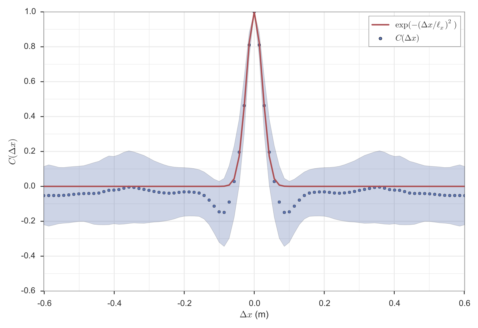
The radial correlation function is fitted with a Gaussian after averaging over time and y:

$C_{fit}(\Delta x) = \exp \left[ - \left(\frac{\Delta x}{\ell_x}\right)^2\right]$

The following is a typical plot resulting from the fit.

Poloidal Fitting¶

The poloidal fitting has two options for fitting controlled using the ky_free configuation parameter:

(Default) Fix $k_y$ to $k_y = 2 \pi / l_y$ and fit using only $\ell_y$ as a free parameter.
Setting ky_free = True will not constrain ky and the fitting procedure will fit using two free parameters.

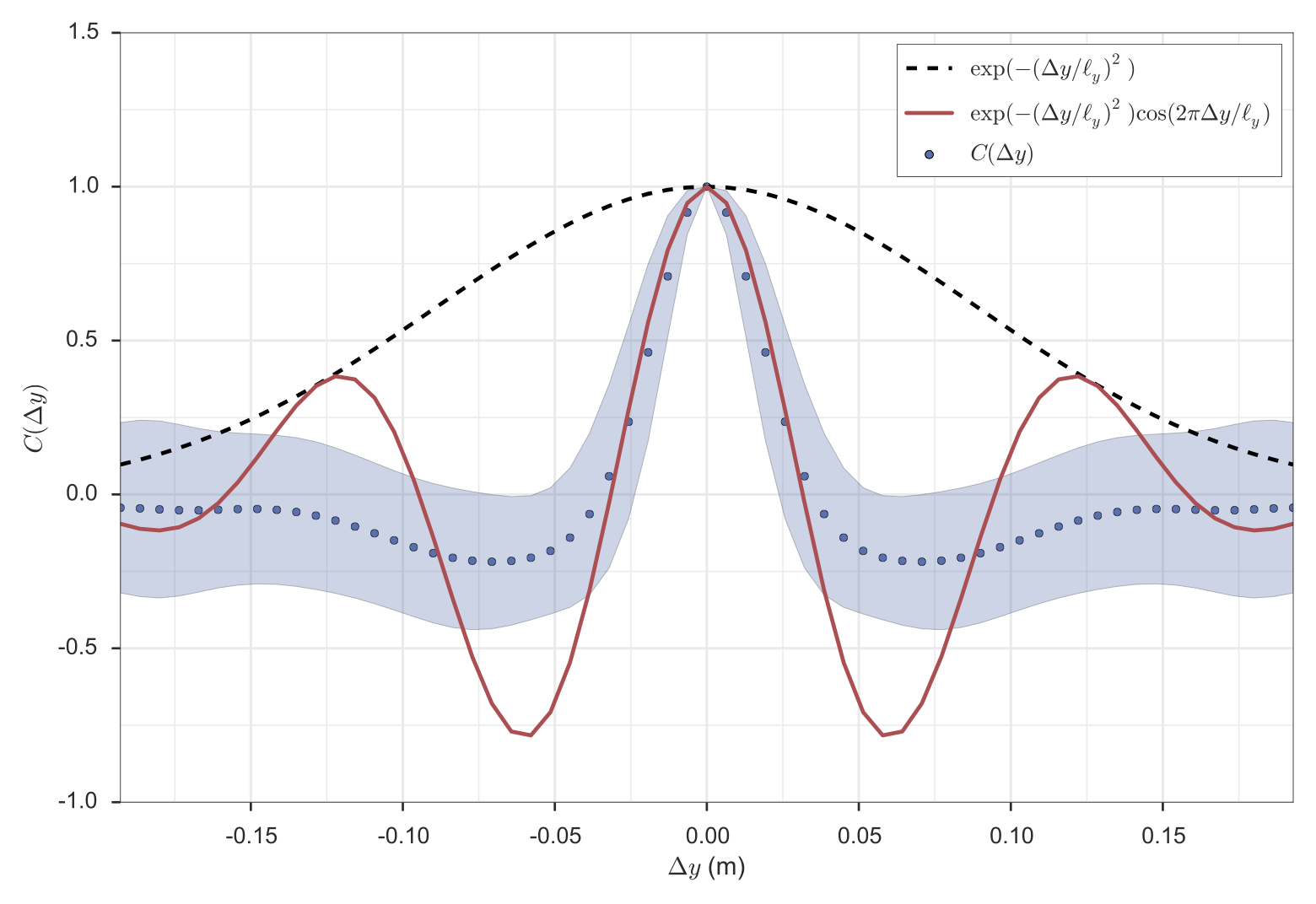
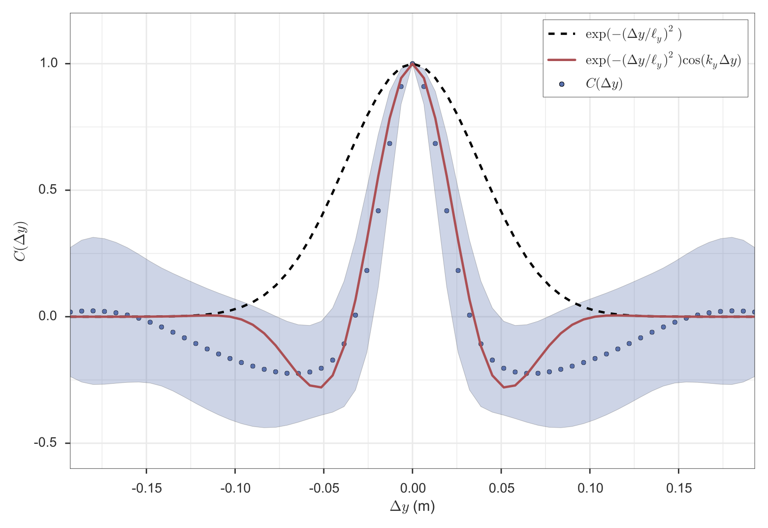
$C_{fit}(\Delta y) = \exp \left[ - \left( \frac{\Delta y}{\ell_y} \right)^2 \right] \cos(k_y \Delta y)$

The following two plots are typical plots resulting from the constrained and unconstrained ky fit, respectively.

The configuration parameter perp_guess typically takes in an array of floats specifying the initial guess for lx and ly. When running with ky as a free parameter it can take a third float specifying the initial guess for ky. Note that the parameter perp_guess is redefined after the first successful fit to be the fitting parameters for that fit.

Time Correlation¶

Calculating the correlation time consists of two main parts:

Calculating the time correlation function.
Fitting the correlation function with an appropriate function to get the correlation time.

Time Correlation Function¶

The field is firstly converted to real space and saved as a new variable called field_real_space. This leaves us with a field f(t, x, y). In order to have some statistics about how the correlation time is changing over the course of the simulation, we split the time domain into time slices, of size time_slice defined in the configuration file. The correlation time may also depend on the size of this time slice, so some tests should be done to ensure that this is understood.

For each time slice we want to calculate the correlation function C(dt, x, dy), leaving us with a function C(it, dt, x, dy), where it denotes the time slice index. This is done by using the SciPy function, scipy.signal.fftconvolve. Noting that a convolution and a correlation calculation is related by a reversal of the indices of the second function.

Fitting¶

The fitting procedure is best illustrated by the following diagram.

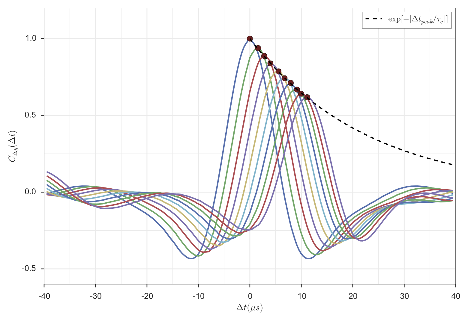
The coloured lines are the correlation function for several different separations in y. The blue line is the decaying exponential fit to the peaks of the correlation function, and the correlation time is the characteristic time of the decaying exponential. Depending on the direction of flow, the peaks may be exponentially increasing or decreasing, and the appropriate function is fitted in either case. In regions where there is no flow, a Gaussian function is fitted to the central, dy = 0, function and the correlation time is taken to be the characteristic time of the exponential envelope.

The following options are relevant to the fitting procedure:

npeaks_fit: determines the number of peaks to fit with a decaying exponential. Having too few or too many may cause the fitting procedure to fail.
time_guess: This is the initial guess used in the fitting procedure in normalized time units. Visual inspection can be used to verify the fitting procedure.

Parallel Correlation¶

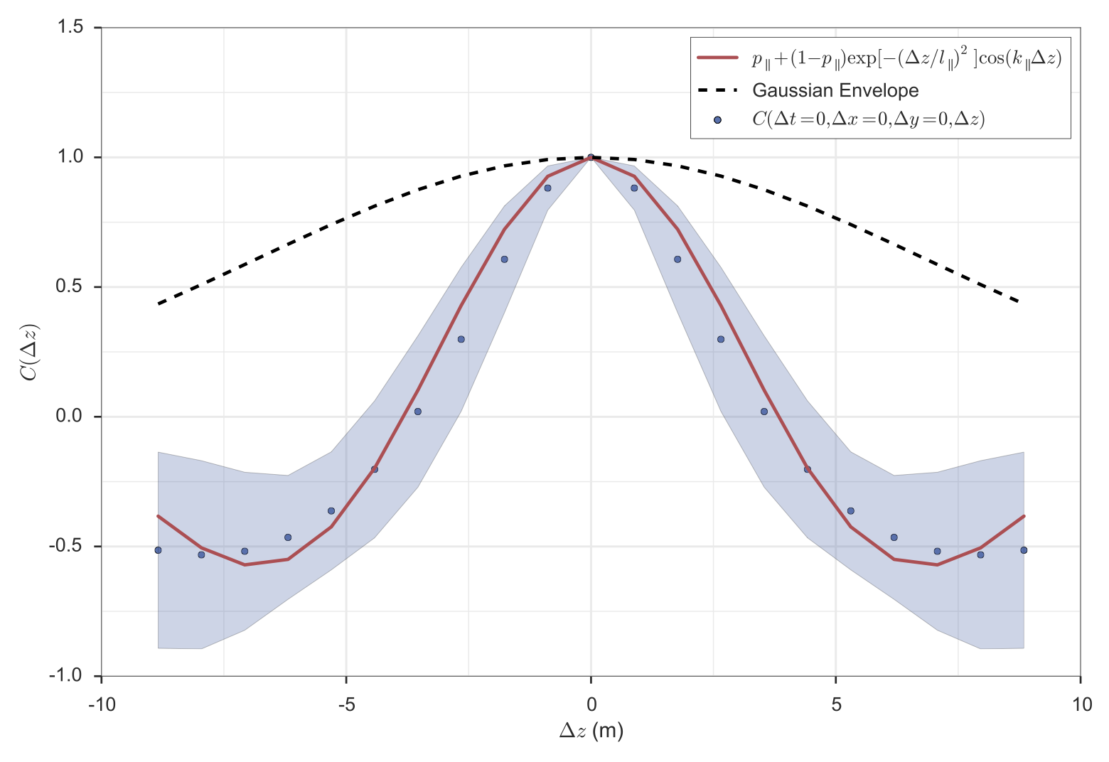
The parallel correlation function fitting is illustrated by the above plot. It involves the following steps:

Loop over x, y, and t to calculate C(t, x, y, dz).
Average over x, y, and t.
Fit C(dz) with an oscillating Gaussian function.

The initial guess for the parallel fit length and wavenumber is set in the par namelist as par_guess. Importantly these numbers should be in metres and metres^-1 since there is no normalized unit in the parallel direction.

Lab Reference Frame¶

Changing to the lab frame involves the following transformation [Holland, PoP 2009]:

$f_{lab}(t, r, n, \theta) = f_{sim}(t, r, n, \theta)e^{-i n \omega_0 t}$

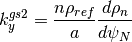
where n is the toroidal wavenumber. The important thing here is that $k_y$ is not the toroidal wavenumber but does have a component in the toroidal direction. The two quantities are related by:

$k_{y}^{gs2} = \frac{n \rho_{ref}}{a} \frac{d \rho_n}{d \psi_N}$

In order to transform to the lab frame, the following configuration quantities are needed:

omega - the angular frequency of the bulk plasma.
dpsi_da - the quantity that relates the GS2 radial grid with the $\psi_N$ grid.

Finally, one can verify that the lab frame transformation has a negligible effect on the perpendicular correlation analysis, however the time correlation analysis will be affected by the transformation. The problem of time resolution becomes immediately apparent since the time resolution is enough to resolve plasma frame quantities but not lab frame quantities. For this reason, time interpolation is almost certainly needed, and a factor four is recommended, following [Holland, PoP 2009]. The level of time interpolation is set using the time_interp_fac configuration variable and a warning is printed out if changing to the lab frame without some time interpolation. The lab frame time correlation analysis is written to a separate folder called ‘time_lab_frame’.